Visualization of complex functions
Multivalued-ness of the the Logarithm
The complex logarithm separates the absolute value and the phase of a complex number,
\[\log z = \log\left(R e^{i\phi}\right)=\log R+i\phi\]The logarithm is the inverse of the exponent, as can be seen from Euler’s formula for example,
\[\exp\big(\log z\big) = \exp^{\log R + i \phi}=R e^{i\phi}=z\]However, the exponent function is not one-to-one, \( \exp(z)=\exp(z+2\pi i k) \) for any integer \(k\). So its inverse is multivalued. That is, there are many possible choices for the angle \(k\). To fix this, \(k\) is conventionally defined to be between \(-\pi\) and \(\pi\), or 0 and \(2\pi\)
This is an arbitrary choice, and it would create a line of discontinuity, called a branch cut. A good way to visualize this is to track a single point and its image under the mapping. Try to drag the blue or red points here:
| | | |
| | Exp Log | |
Things to try/notice:
- Note that when dragging the red point, the blue point always moves continuously. However, when dragging the blue point in branch cut mode, the red point jumps discontinuously when crossing the branch cut.
- Drag the blue point in a small path that does not encircle the origin.
- Drag the blue point in a small path that encircles the origin. Try both clockwise and anti-clockwise, in the branch-cut or multi-valued modes.
- Try to drag the red dot such that the blue dot follows a vertical/horizontal line. Did you see that the mapping \( z\to \log z\) is very similar to a coordinate transform from cartesian to polar coordinates?
Another way of thinking about a multivalued function is a Riemann surface, which informally is the “stiching together” of the multiple values (“branches”) of the inversion problem. Here you can see the real and imaginary part of the logarithm Riemann surface. That is, we plot \(\mbox{Re}(\log(x+iy))\) and \(\mbox{Im}(\log(x+iy))\) as functions of \(x,y\). 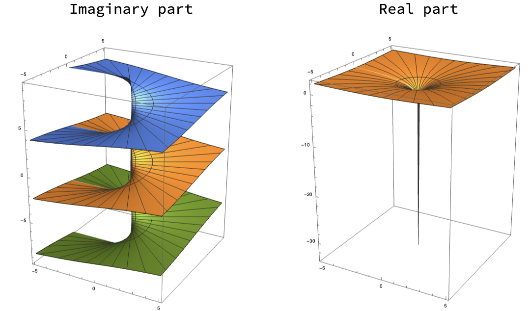 The choice \(-\pi<\phi<\pi\) corresponds to the yellow sheet.
Another insightful visualization is the deformation of the gridlines under the log function. In this widget, every point \(z\) moves on a straight line from its “original” position at \(t=0\) to \(\exp(z)\) at \(t=1\):
Note that when you go from \(t=1\) to \(t=0\), you’re looking at how the logarithm (which is the inverse of the exponent) warps the complex plane. That is, how it takes a polar grid and returns a cartesian one.
Powers and roots
A similar thing happens for powers and roots. Let’s look for example at the function \( z\to z^2 \) and its inverse, \( z\to\sqrt z \). In polar representation, \( z=Re^{i\theta} \), the square function squares the radius and doubles the angle. Try to drag the red dot in a circle around the origin, and see what happens to the blue dot:
| | ||
| | Square Square root | |
Here again you see that the map \( z\to z^2 \) is nice and smooth and has no discontinuities, but its inverse map \( z\to\sqrt z \) is either multivalued or has a branch cut. this is because \( z\to z^2 \) wraps the plane around itself twice:
Note how the result is independent of the choice of branch cut when α is an integer. In this case, the complex plane maps onto itself exactly α times. When \(\alpha\) is an integer, the branch cut exactly closes off. Actually, raising to the power \( \alpha \) is defined by \( z^\alpha = e^{\alpha \log z}\). So the branch cut in the sqrt function, or any other fractional power, is the same branch cut of the imaginary part of the logarithm.